Three-body interactions pose a challenging inverse problem. A trajectory records the combined acceleration from all active forces, while a genuinely non-additive term cannot be reconstructed by summing pairwise fits. The Axilrod-Teller triple-dipole potential provides a demanding test: its energy scales as r^-9, its force as r^-10, and its angular factor changes sign between compact and elongated triangles. The paper asks whether motion alone can reveal this hidden law.
Sena Kalabalık and colleagues prescribe the kinetic energy exactly and train a neural network to represent only the unknown position-dependent potential. They use pairwise distances and the cosines of the three interior angles as a symmetry-adapted representation. Automatic differentiation converts the learned scalar potential into accelerations, allowing training on position-acceleration pairs rather than energy or potential labels. The study tests the recovered field, its radial and angular structure, trajectory rollouts, identifiability against a Lennard-Jones background, and symbolic recovery of the analytic law.
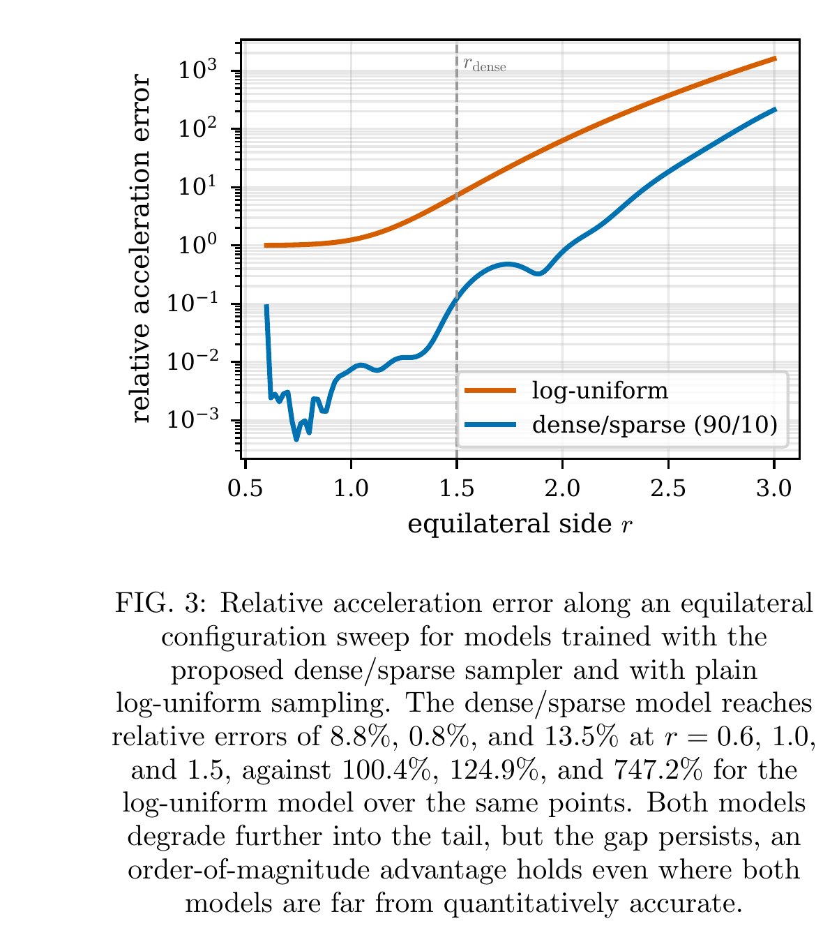
The clearest controlled result is about data allocation. The authors use 120,000 training configurations and 24,000 validation configurations. Their dense/sparse sampler places 84% of configurations where at least two dimensionless separations are below r_dense = 1.5, compared with 28% for plain log-uniform sampling. Along an equilateral sweep, Figure 3 reports relative acceleration errors of 8.8%, 0.8%, and 13.5% at dimensionless r = 0.6, 1.0, and 1.5. At those same points, the matched log-uniform model reaches 100.4%, 124.9%, and 747.2%. At r = 1.0, the proposed sampling reduces the reported error by a factor of about 156.
This result has relevance beyond the analytic benchmark because inverse identification is often constrained by where measurements are collected, not just by model capacity. When a force varies over orders of magnitude, uniform coverage of a coordinate range may still undersample the region that determines the law. The structured network also supports symbolic regression: the recovered expression retains the angular numerator, the r^-9 radial dependence, and a coupling near one, with R^2 approximately 0.98 against the analytic potential after the unphysical additive constant is removed.
The limitations are decisive. The dynamics are entirely synthetic and use reduced Lennard-Jones units; the authors explicitly make no claim that this is a quantitatively realistic material model. The Axilrod-Teller term is an asymptotic long-range approximation and becomes incomplete at short separation. More importantly, at the argon-like dimensionless coupling of about 0.1, the three-body acceleration has a median magnitude of about 0.009 in reduced acceleration units—five times below the pairwise model's error floor of about 0.045—and is below that floor for 85% of configurations. With the selected architecture and data budget, the physically scaled term is not identifiable. The method also assumes a position-only potential and a constant mass matrix.
Proposed ten-business-day pilot
This is a proposed feasibility study, not a completed experiment or a claim of novelty.
- Days 1–2 — Freeze the inverse problem and inputs. Use a public three-particle trajectory generator with a known pairwise baseline and one withheld three-body term. Version the equations, nondimensionalization, integrator, time step, initial-condition bounds, noise model, and random seeds. Generate positions and independently compute accelerations using a higher-order finite-difference stencil or analytic derivatives for validation only.
- Days 3–4 — Establish the baseline. Fit a pairwise neural potential and a fully learned Lagrangian network to the same position-acceleration budget. Use a fixed random split and a geometry-blocked holdout that excludes one range of triangle shapes. Record acceleration MAE in reduced units, relative L1 error, rollout position error, energy drift, and training time in hours.
- Days 5–6 — Add structured three-body recovery. Prescribe the kinetic term, provide distance and angle features, and train the position-only potential. Compare log-uniform sampling with a pre-registered dense/sparse mixture, keeping architecture, optimizer, sample count, and seeds fixed. Keep the analytic potential hidden from training.
- Days 7–8 — Validate independently. Evaluate both samplers on the blocked geometries, an equilateral sweep, and at least 100 rollout initial conditions. Test three coupling levels spanning below, near, and above the baseline error floor. Use a separate script to verify permutation, translation, and rotation invariance and compare gradients against analytic accelerations.
- Days 9–10 — Stress-test and package. Introduce one controlled acceleration-noise level, repeat the symbolic-regression stage both with and without angle features, and report failures as well as successes. Deliver locked dependencies, immutable data manifests, configuration files, seeds, raw metrics, trained checkpoints, all validation outputs, and a one-command rebuild of the figure and table.
The resulting reproducible evidence could support a later study and, if warranted by the findings, a future manuscript. It does not claim that the implementation, validation, novelty assessment, or publication already exists.
