Engineering design rarely begins with a blank sheet. A turbine blade, magnetic coil set, or load-bearing component may need an improved objective value while preserving a trusted state, such as lift, boundary shape, or modal response. When an expensive partial-differential-equation solver produces that state, standard constrained Bayesian optimisation must learn a thin, highly anisotropic feasible set from scarce scalar observations. As a result, many early candidates may be infeasible before the optimizer has learned where useful designs lie.
Gabriel Diaz-Aylwin and colleagues encode the preservation constraint in the proposal geometry. They linearise the selected state observable around the baseline, map its tolerance back into design space through the response Jacobian, and thereby obtain an ellipsoidal feasible region. Ray-intersection sampling and maximin filtering yield well-spread candidates within this region. After each simulator evaluation, the response map is refitted, while a low-rank field model estimates residual nonlinear changes and allows acquisition refinement beyond the linearised boundary.
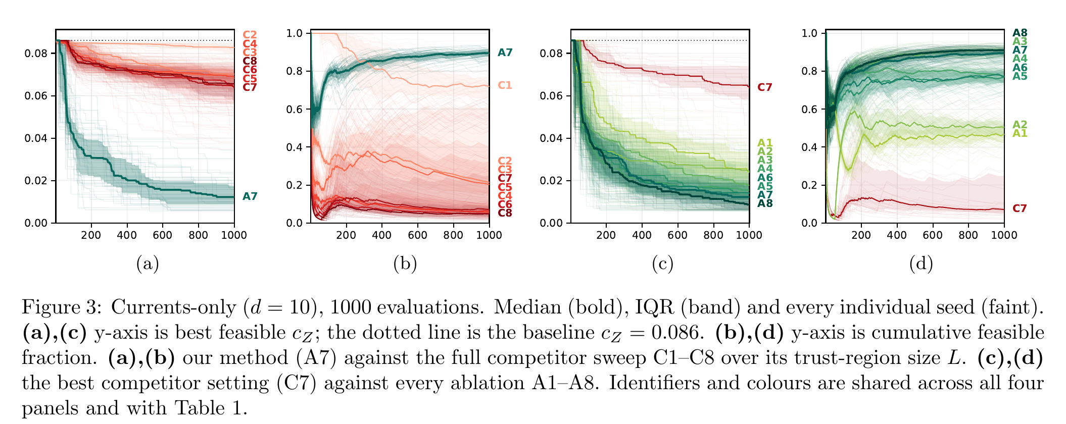
The currents-only tokamak benchmark offers the clearest quantitative comparison. Across 50 seeds and a matched budget of 1,000 evaluations, the full method achieved a median final detachment-threshold impurity fraction c_Z of 0.0122, compared with 0.0636 for the best reported competitor setting—a 5.2-fold reduction. The impurity fraction is dimensionless. Meanwhile, 89.5% of the full method's evaluations met the 0.5 cm last-closed-flux-surface displacement tolerance, compared with 7.1% for that competitor. Figure 3 presents the median, interquartile range, and individual runs. The initial finite-difference Jacobian required 20 additional solver calls, which were not included in the matched 1,000-evaluation budget.
This matters because preservation constraints are not ordinary black-box inequalities. Their local geometry is encoded in how a high-dimensional state responds to design perturbations. A small, explicit Jacobian budget can expose that geometry and prevent an expensive optimizer from having to rediscover it through successive failed evaluations. The same proposal mechanism can be used with different acquisition functions; the paper demonstrates a two-objective extension that replaces expected improvement with expected hypervolume improvement.
The evidence is still application-specific. The experiments couple FreeGSNKE equilibrium calculations with FusionDLS rather than a physical tokamak experiment, and the main comparisons address one simulated divertor-design workflow. The multi-objective demonstration does not include a competing multi-objective trust-region baseline. The method also requires a usable baseline Jacobian, and its linearisation can deteriorate as the search moves away from that baseline. In the 30-variable test, a frozen map yielded a median violation-prediction error of 1.07 cm, exceeding the 0.5 cm tolerance; online refitting lowered the held-out one-step-ahead median error to 0.031 cm. These results indicate a promising optimization strategy, not guaranteed transfer to another engineering system.
Proposed ten-business-day pilot
This would be a proposed feasibility study, not a completed experiment or a claim of novelty.
- Days 1–2 — Freeze the problem and inputs. Choose one finite-element bracket or thermal component with 8–12 continuous design variables. Version the mesh, material law, loads, solver tolerances, and baseline state. Define one objective, such as mass or peak temperature, and one preserved observable, such as the first three modal frequencies or a boundary-temperature field. Set the preservation tolerance before optimization and reserve an independently refined mesh for validation.
- Days 3–4 — Establish the baseline. Implement constrained Bayesian optimisation using a Gaussian-process model of scalar violation. Use the same initial design, acquisition function, and 150 expensive evaluations planned for the proposed method. Record every solver failure and feasible evaluation.
- Days 5–6 — Add state-aware proposals. Estimate the response Jacobian with centered finite differences, construct the pulled-back ellipsoid, and implement ray-intersection sampling with maximin filtering. Track finite-difference calls separately in the cost ledger. Refit the response map using only data available at each iteration.
- Days 7–8 — Validate independently. Run both methods with at least five fixed seeds. Re-solve each claimed optimum on the held-out refined mesh and compare the preserved field or modal quantities without retuning. Measure objective improvement in %, feasible-evaluation fraction in %, normalized RMS state displacement, state-prediction error, wall-clock time in h, and failed-solve count. If including an optional second objective, report hypervolume and Pareto-set feasibility while keeping the single-objective comparison as the primary baseline.
- Days 9–10 — Stress-test and package. Vary the state tolerance and finite-difference step once, document linearisation failures, and regenerate all tables and figures with a single command. Deliver the source code, locked dependencies, immutable inputs, seed manifests, solver logs, raw metrics, validation outputs, and a concise methods-and-results note.
The resulting reproducible evidence could support a later study and, if warranted by the findings, a future manuscript. It does not claim that the implementation, validation, novelty assessment, or publication already exists.
