A deterministic surrogate assumes that each operating condition maps to a single response. Symmetry-breaking bifurcations violate this assumption: beyond a critical point, the same geometry, loading path, and initial state can produce several equally valid trajectories. A model trained with a pointwise loss may average these branches into a response that is not physically admissible. This poses a serious problem for digital twins designed to explore post-buckling structures, phase separation, or other multistable systems.
Bi-FORK, introduced by Anna Zimmel and colleagues, represents the response as a conditional distribution rather than a single field. An encoder first compresses the full space-time trajectory, after which latent flow matching generates complete trajectories jointly, preserving branch coherence across space and time. During inference, repulsion-guided sampling steers concurrent samples toward distinct branches after the predicted bifurcation point. The method is evaluated on three different symmetry-breaking systems: three-dimensional beam buckling, periodic mechanical metamaterials, and three-dimensional Allen–Cahn phase separation, with discretizations reaching 260,000 points.
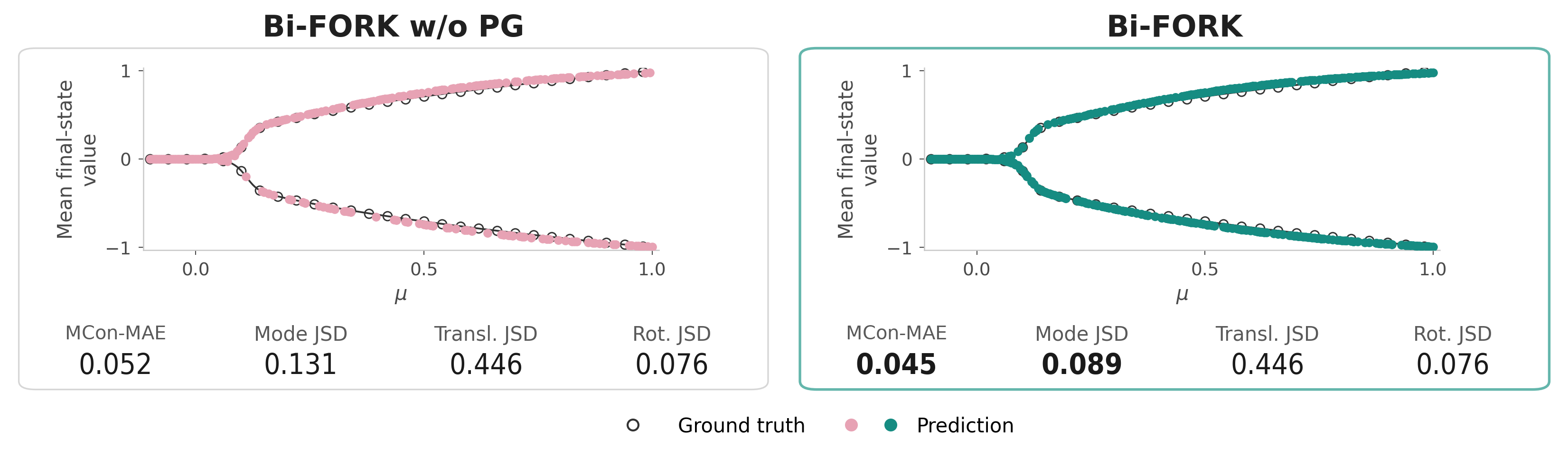
The Allen–Cahn experiment provides a useful quantitative check. Across five evaluation seeds, adding particle guidance reduced the relaxed, mode-conditioned mean absolute error from 0.0515 ± 0.001 to 0.0453 ± 0.000, a 12.0% reduction. It also reduced the dimensionless mode-coverage Jensen–Shannon divergence from 0.131 ± 0.010 to 0.089 ± 0.001, a 32.1% reduction. Both metrics are dimensionless. Figure 7 shows the corresponding branch recovery across the dimensionless control parameter μ. On the smaller Beam3D benchmark, Bi-FORK generated 180 samples for one condition in 3.95 s on a single NVIDIA B300 SXM6 GPU, compared with 72.32 s for STFlow and 7,766.36 s for GeoTDM; these timings should not be generalized beyond the reported hardware and workloads.
This result matters because a useful branch-aware digital twin must represent alternative futures while preserving spatial and temporal consistency. Bi-FORK provides a practical mechanism for doing so at dimensions where repeated continuation, deflation, or stochastic solvers can become expensive. The work also makes evaluation more physically informative by measuring whole-trajectory accuracy, rejection from the solution manifold, and coverage of symmetry-related modes, rather than relying solely on pointwise error.
The limitations are equally important. Particle guidance may trade accuracy for diversity by pushing samples that are already valid away from the solution manifold. The Allen–Cahn distribution is not exhaustively known: mode coverage is estimated from four simulated realizations per condition and their sign flips, while separate mode, translation, and rotoreflection divergences do not certify the joint distribution. Symmetry is learned through data and augmentation rather than enforced by the architecture. For the largest systems, no existing stochastic baseline scaled to the task, so the comparison is limited to a deterministic affine baseline and Bi-FORK ablations. These results therefore demonstrate a promising surrogate strategy, not a universal solution to bifurcation analysis.
How I'd pilot this in 10 business days
- Days 1–2 — Freeze the system and evidence. Select one slender structure or periodic lattice with two or four known post-buckling branches. Version the mesh, material parameters, boundary conditions, load path, continuation settings, and random seeds. Reserve complete geometries—not individual frames—for the validation and test sets.
- Days 3–4 — Establish independent baselines. Use a trusted finite-element continuation or deflation solver to recover reference branches. Train a deterministic mean predictor and a stochastic model without particle guidance. Record dimensionless mode-conditioned MAE and Jensen–Shannon divergence, branch coverage in %, rejected trajectories in %, wall-clock time in s, and peak GPU memory in GB.
- Days 5–6 — Implement the branch-aware surrogate. Train the trajectory autoencoder and latent flow-matching model on the frozen training geometries. Add bifurcation-time prediction and repulsion-guided sampling without changing the held-out sets. Keep model checkpoints, configurations, dependency locks, and seed manifests under version control.
- Days 7–8 — Validate independently. For unseen geometries and load paths, compare every generated trajectory with solver-relaxed or continuation-derived branches. Test whether guidance improves coverage without an unacceptable increase in error or rejection rate. Repeat the evaluation across at least five fixed seeds and report uncertainty, not just the best run.
- Days 9–10 — Stress-test and package. Vary sample count and guidance strength, document failure cases near the critical point, and reproduce all tables and figures with a single command. Deliver code, an environment lockfile, immutable inputs, solver logs, trained checkpoints, evaluation outputs, and a concise methods-and-results note.
This is a proposed feasibility study. Its reproducible evidence could support a later investigation and manuscript, but it does not claim that the implementation, experiments, validation, novelty assessment, or publication already exists.
