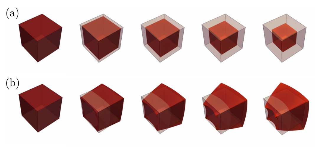
A vanishing bulk stiffness can expose deformation patterns that a uniform compression test would miss. In their 13 October preprint, Franke, Sander and Garst analyze linear elasticity without externally applied stress. At an isostructural instability, they identify four non-rigid critical modes: one dilation and three special conformal transformations. Six rigid translations and rotations are distinct from these modes. These counts describe modes, not measured material properties.
For mechanical metamaterials, the analysis suggests testing spatial deformation patterns as well as effective stiffness. Its scope is important: strain-gradient terms and nonlinear response add energy costs. The paper does not establish the absorption performance of any manufactured device.
Proposed ten-business-day pilot
This is an original computational study proposal. It has not been carried out and makes no claim of novelty or of a publication-ready result.
- Days 1–2: define a reproducible benchmark. Specify a traction-free three-dimensional cube, a positive reference shear modulus, density, length scale, and a sequence of decreasing positive bulk-to-shear ratios. Record units, mesh-generation details, quadrature, and solver tolerances. Set a small displacement amplitude and a testable convergence criterion before calculating results.
- Days 3–4: establish the numerical baseline. Assemble a fully integrated quadratic finite-element model and its mass matrix. Remove rigid-body motion by projection rather than by clamping arbitrary nodes. Solve the generalized eigenproblem and record normalized eigenvalues, residual norms, and execution time. Repeat on three meshes and compare against a stable material far from the soft limit.
- Days 5–6: compare independent descriptions. Implement the published analytical displacement fields in a separate script. Directly check their strains and surface tractions, then compare their span with the numerical low-energy subspace using principal angles. Track subspaces instead of assigning physical meaning to the basis returned by an eigensolver within a degenerate eigenspace.
- Days 7–8: test the apparent agreement. Repeat using different mesh orientations and element orders, checking for under-integration artifacts. Add a small, explicitly documented boundary restraint as a sensitivity case, separate from the traction-free benchmark. Report eigenvalue ratios, subspace errors, residuals, and convergence trends without prescribing a desired answer.
- Days 9–10: package evidence and limitations. Archive input files, dependency versions, meshes, raw matrices or reproducible assembly instructions, solver outputs, and plotting scripts. Prepare a table distinguishing analytical predictions, numerical observations, and unresolved discrepancies. Provide a single command that reproduces all reported comparisons.
Whether to pursue a later experiment would depend on stable convergence, agreement between independent implementations, and a clear account of boundary sensitivity. This pilot alone would neither validate a fabricated material nor demonstrate energy absorption.
